Exploring ChIP-seq Data with ChIPseeker: An Essential Tool for Peak Annotation
Peak annotation in ChIP-seq data analysis involves identifying genomic features associated with regions of significant enrichment (peaks), such as genes, promoters, enhancers, or other regulatory elements. This process is crucial for understanding the biological significance of the data by linking DNA-protein interactions to specific functional genomic regions. ChIPseeker is a popular R package designed for the annotation and visualization of ChIP-seq data. It supports multiple genome annotations and can be easily integrated with other bioinformatics tools, enhancing its utility. A key strength of ChIPseeker is its ability to provide detailed annotation of peaks with respect to nearest genes and genomic features, along with comprehensive visualization options like pie charts and histograms that summarize the genomic distribution of the peaks. This protocol was created based on ChIPseeker version 1.32.1 running on a system equipped with an Intel 10th generation i9-10910 processor and 48GB of memory. The test environment includes R version 4.4.0 under macOS 12.4 environment.
Installation ChIPseeker
1. Check and install ChIPseeker
Start by ensuring the BiocManager package is installed, then install ChIPseeker using it:
  if (!requireNamespace("BiocManager", quietly=TRUE))
      install.packages("BiocManager")
  ## BiocManager::install("BiocUpgrade") ## you may need this
  BiocManager::install("ChIPseeker")
2. Install Required Libraries
Install additional libraries necessary for ChIPseeker to function properly. These include packages for genomic data manipulation and annotation. You can install these packages manually using the
BiocManager::install("<PackageName>"). The list of packages is shown below.Dependency list
GenomeInfoDb: Utilities for manipulating chromosome namesGenomicRanges: Representation and manipulation of genomic intervalsGenomicFeatures: Conveniently import and query gene modelsrtracklayer: R interface to genome annotation files and the UCSC genome browserclusterProfiler: statistical analysis and visualization of functional profiles for genes and gene clustersAnnotationDbi: Manipulation of SQLite-based annotations
Genome data list (Note, it depends on the species you want to analyze. In this manual, I only provide the analysis of human and mouse genome.)
TxDb.Mmusculus.UCSC.mm10.knownGene: Annotation package for TxDb objects for mouseTxDb.Hsapiens.UCSC.hg19.knownGene: Annotation package for TxDb objects for humanEnsDb.Mmusculus.v79: Ensembl based annotation package for mouseEnsDb.Hsapiens.v86: Ensembl based annotation package for humanorg.Mm.eg.db: Genome wide annotation for Mouseorg.Hs.eg.db: Genome wide annotation for human
Critical Note
Before installing each package, check if it is already installed and only install those that are missing. This can save time and avoid unnecessary installations. Here is how you can check and install a package only if it’s not already installed:
  install_if_missing <- function(package_name) {
      if (!requireNamespace(package_name, quietly = TRUE)) {
          BiocManager::install(package_name)
      } else {
          message(paste(package_name, "is already installed."))
      }
  }

  # List of dependencies
  dependencies <- c("GenomeInfoDb", "GenomicRanges", "GenomicFeatures",
                  "rtracklayer", "clusterProfiler", "AnnotationDbi")

  # Install dependencies one by one
  lapply(dependencies, install_if_missing)

  # List of genome data packages (Optional)
  genome_data <- c("TxDb.Mmusculus.UCSC.mm10.knownGene",
                  "TxDb.Hsapiens.UCSC.hg19.knownGene",
                  "EnsDb.Mmusculus.v79", "EnsDb.Hsapiens.v86",
                  "org.Mm.eg.db", "org.Hs.eg.db")

  # Install genome data packages one by one
  lapply(genome_data, install_if_missing)
Step-by-step Running Guide ChIPseeker
1. Load ChIPseeker and its dependency packages
library(ChIPseeker)
library(TxDb.Hsapiens.UCSC.hg19.knownGene)
library(EnsDb.Hsapiens.v86)
library(clusterProfiler)
library(AnnotationDbi)
library(org.Hs.eg.db)
library(ggplot2)
library(ggupset)
library(ggplotify)
library(ggimage)
library(RColorBrewer)
2. Load peak data
In this course, I will use peak data acquired with SICER. When using data acquired with MACS, you can load
narrow,broad, orbedfiles as you see fit for your analysis.Sicer_H3K4me3 <- readPeakFile("/Users/jchoi/Desktop/Unt_H3K4me3-W50-G100-islands-summary", header = F) Sicer_H3K27me3 <- readPeakFile("/Users/jchoi/Desktop/Unt_H3K27me3-W50-G100-islands-summary", header = F) Sicer_MLL1 <- readPeakFile("/Users/jchoi/Desktop/Unt_MLL1-W50-G100-islands-summary", header = F) Sicer_UTX <- readPeakFile("/Users/jchoi/Desktop/Unt_UTX-W50-G100-islands-summary", header = F) peaks <- list(H3K4me3 = Sicer_H3K4me3, H3K27me3 = Sicer_H3K27me3, MLL1 = Sicer_MLL1, UTX = Sicer_UTX) peaks
- Output:
  > peaks
  $H3K4me3
  GRanges object with 59583 ranges and 5 metadata columns:
          seqnames            ranges strand |        V4        V5           V6         V7           V8
              <Rle>         <IRanges>  <Rle> | <integer> <integer>    <numeric>  <numeric>    <numeric>
      [1]     chr1       10051-10599      * |        53        68    1.0000000   0.924306    1.0000000
      [2]     chr1       11601-14399      * |       171       181    0.0653982   1.120382    0.0695043
      [3]     chr1       14551-15249      * |        34        28    0.0166897   1.440023    0.0182155
      [4]     chr1       15401-17099      * |        73        77    0.1441852   1.124296    0.1513844
      [5]     chr1       17251-18049      * |        38        64    1.0000000   0.704129    1.0000000
      ...      ...               ...    ... .       ...       ...          ...        ...          ...
  [59579]     chrY 59011501-59026949      * |      1413       778 7.55580e-145  2.1538291 4.09978e-144
  [59580]     chrY 59027151-59033299      * |       552       225 1.81527e-101  2.9094120 8.81781e-101
  [59581]     chrY 59213451-59214949      * |        75         5  2.58202e-66 17.7885247  1.10346e-65
  [59582]     chrY 59362851-59363399      * |        25        46  1.00000e+00  0.6445118  1.00000e+00
  [59583]     chrM       12351-13249      * |        39      1856  1.00000e+00  0.0249193  1.00000e+00
  -------
  seqinfo: 25 sequences from an unspecified genome; no seqlengths

  $H3K27me3
  GRanges object with 93824 ranges and 5 metadata columns:
          seqnames      ranges strand |        V4        V5          V6        V7          V8
              <Rle>   <IRanges>  <Rle> | <integer> <integer>   <numeric> <numeric>   <numeric>
      [1]     chr1 31101-31849      * |        41        11 7.52852e-14   4.02644 2.02150e-13
      [2]     chr1 32601-33349      * |        32        13 4.73028e-07   2.65911 7.00814e-07
      [3]     chr1 33701-34499      * |        54        23 8.04691e-10   2.53627 1.53203e-09
      [4]     chr1 34651-35399      * |        40        11 3.12778e-13   3.92823 7.96170e-13
      [5]     chr1 35651-36349      * |        54        11 9.84610e-23   5.30312 4.90046e-22
      ...      ...         ...    ... .       ...       ...         ...       ...         ...
  [93820]     chrM   4751-5899      * |        62      2070           1 0.0323557           1
  [93821]     chrM   6051-6999      * |        46      1885           1 0.0263619           1
  [93822]     chrM  7151-10949      * |       187      6820           1 0.0296202           1
  [93823]     chrM 11101-14399      * |       202      6535           1 0.0333915           1
  [93824]     chrM 14551-16549      * |       131      3655           1 0.0387181           1
  -------
  seqinfo: 25 sequences from an unspecified genome; no seqlengths

  $MLL1
  GRanges object with 34003 ranges and 5 metadata columns:
          seqnames            ranges strand |        V4        V5          V6        V7          V8
              <Rle>         <IRanges>  <Rle> | <integer> <integer>   <numeric> <numeric>   <numeric>
      [1]     chr1       10001-10499      * |        51        63   1.0000000  0.780916   1.0000000
      [2]     chr1       11901-13049      * |        60        92   1.0000000  0.629126   1.0000000
      [3]     chr1       16901-17299      * |        31        22   0.0397828  1.359294   0.0557065
      [4]     chr1       17451-18099      * |        36        49   1.0000000  0.708730   1.0000000
      [5]     chr1       19851-20799      * |        39        44   1.0000000  0.855040   1.0000000
      ...      ...               ...    ... .       ...       ...         ...       ...         ...
  [33999]     chrY 59029651-59030999      * |        91        52 1.48881e-06  1.688156 5.32648e-06
  [34000]     chrY 59031151-59032099      * |        68        30 3.24751e-09  2.186563 2.14925e-08
  [34001]     chrY 59032401-59033199      * |        36        70 1.00000e+00  0.496111 1.00000e+00
  [34002]     chrY 59362951-59363399      * |        85        44 6.37554e-08  1.863548 3.07182e-07
  [34003]     chrM           1-16549      * |      7206     29637 1.00000e+00  0.234549 1.00000e+00
  -------
  seqinfo: 25 sequences from an unspecified genome; no seqlengths

  $UTX
  GRanges object with 44845 ranges and 5 metadata columns:
          seqnames            ranges strand |        V4        V5          V6        V7          V8
              <Rle>         <IRanges>  <Rle> | <integer> <integer>   <numeric> <numeric>   <numeric>
      [1]     chr1       10051-10449      * |        58        59 0.161707386  1.127780 0.178211140
      [2]     chr1       13301-13899      * |        32        35 0.349485362  1.048891 0.373021173
      [3]     chr1       14551-15249      * |        26        28 0.325894887  1.065279 0.348971602
      [4]     chr1       16851-17799      * |        47        76 1.000000000  0.709467 1.000000000
      [5]     chr1       19101-20649      * |        70        53 0.000421408  1.515202 0.000653707
      ...      ...               ...    ... .       ...       ...         ...       ...         ...
  [44841]     chrY 59028701-59029749      * |        40        32 1.17852e-02  1.434030 1.48488e-02
  [44842]     chrY 59030051-59030599      * |        42        24 1.55131e-05  2.007642 3.07036e-05
  [44843]     chrY 59030851-59032599      * |        85        59 6.65690e-06  1.652780 1.41208e-05
  [44844]     chrY 59362901-59363399      * |        45        45 1.57970e-01  1.147224 1.74366e-01
  [44845]     chrM           1-16549      * |      4103     29637 1.00000e+00  0.158824 1.00000e+00
  -------
  seqinfo: 25 sequences from an unspecified genome; no seqlengths
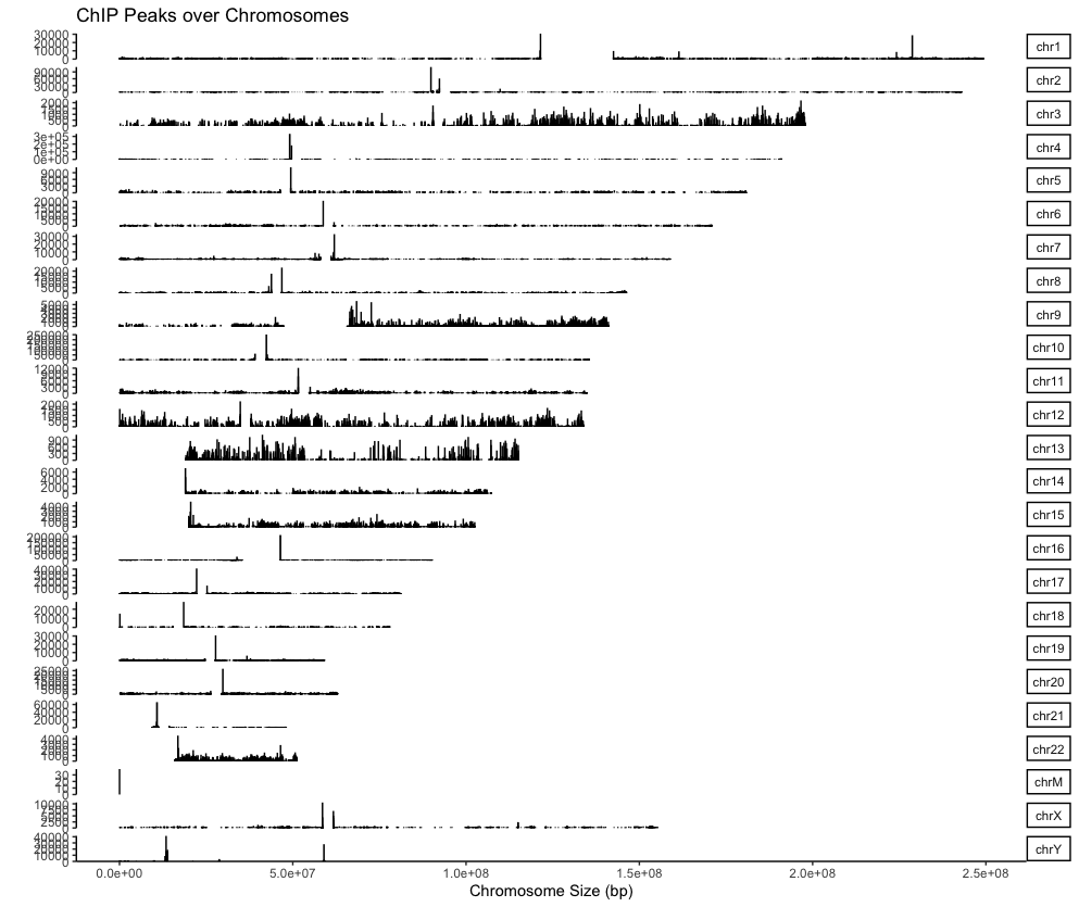
3. Make coverage plot
Before depict coverage plot, it is important to understand the structure of the
peaksobjects: make sure you know what each column means. The output of ‘sicer’ is chromosome (V1; seqnames), start (V2; ranges), end (V2; ranges), strand (V3; strand), ChIP_signal (V4), Input_signal (V5), p-val (V6), fold change (V7), fdr (V8), in that order. This means that to draw a coverage plot, you will need values from V4 or V7.covplot(peaks[["H3K4me3"]], weightCol="V4") # To save the plot, use 'Export' in the 'Plots' section on the right. covplot(peaks[["H3K27me3"]], weightCol="V4") covplot(peaks[["MLL1"]], weightCol="V4") covplot(peaks[["UTX"]], weightCol="V4") # Can be selected specific chromosomes as follow: covplot(peaks[["H3K4me3"]], weightCol="V4", chrs=c("chr3", "chr4"))Output:
4. Profile of ChIP peaks binding to TSS regions
For calculating the profile of ChIP peaks binding to TSS regions, prepare the TSS regions, which are defined as the flanking sequence of the TSS sites. Then align the peaks that are mapping to these regions, and generate the tagMatrix:
txdb <- TxDb.Hsapiens.UCSC.hg19.knownGene promoter <- getPromoters(TxDb=txdb, upstream=3000, downstream=3000) tagMatrixList <- lapply(as.list(peaks), getTagMatrix, windows=promoter)- Output:
> txdb <- TxDb.Hsapiens.UCSC.hg19.knownGene > promoter <- getPromoters(TxDb=txdb, upstream=3000, downstream=3000) > tagMatrixList <- lapply(as.list(peaks), getTagMatrix, windows=promoter) >> preparing start_site regions by gene... 2024-05-21 12:41:47 >> preparing tag matrix... 2024-05-21 12:41:47 >> preparing start_site regions by gene... 2024-05-21 12:41:56 >> preparing tag matrix... 2024-05-21 12:41:56 >> preparing start_site regions by gene... 2024-05-21 12:42:01 >> preparing tag matrix... 2024-05-21 12:42:01 >> preparing start_site regions by gene... 2024-05-21 12:42:06 >> preparing tag matrix... 2024-05-21 12:42:06 - Heatmap of ChIP binding to TSS regions
  # Multiplot
  peakHeatmap(peaks, TxDb = txdb, nbin = 100, upstream = 3000, downstream = 3000,
              by = "gene", type = "start_site", palette = "Reds")

  # Individual plot
  peakHeatmap(peaks[["PeakName"]], TxDb = txdb, nbin = 100, upstream = 3000, downstream = 3000,
              by = "gene", type = "start_site", palette = "Reds")
In these arguments,
Parameter Description peaksPath to the peak file or a GRanges object containing peak information. TxDbTranscript Database (TxDb) object. nbinNumber of bins to use for drawing the heatmap. Determines the resolution of the heatmap. The lower the nbinvalue, the faster the processing, but the lower the image quality.upstream,downstreamDistance upstream and downstream of the TSS, respectively. byCategory to base the peak heatmap on. Possible values are gene,transcript,exon,intron,3UTR,5UTR, andUTR.typeSpecifies genomic regions to heatmap. Possible values are start_site(tss),end_site(tes),body(gene body).paletteColor palette for the heatmap.
- Output:
  > peakHeatmap(peaks, TxDb = txdb, nbin = 100, upstream = 3000, downstream = 3000,
              by = "gene", type = "start_site", palette = "Reds")
  >> preparing promoter regions...	 2024-05-21 14:38:23
  >> preparing tag matrix...		 2024-05-21 14:38:23
  >> binning method is used...2024-05-21 14:38:23
  >> preparing start_site regions by gene... 2024-05-21 14:38:23
  >> preparing tag matrix by binning...  2024-05-21 14:38:23
  >> binning method is used...2024-05-21 14:38:40
  >> preparing start_site regions by gene... 2024-05-21 14:38:40
  >> preparing tag matrix by binning...  2024-05-21 14:38:40
  >> binning method is used...2024-05-21 14:38:47
  >> preparing start_site regions by gene... 2024-05-21 14:38:47
  >> preparing tag matrix by binning...  2024-05-21 14:38:47
  >> binning method is used...2024-05-21 14:38:51
  >> preparing start_site regions by gene... 2024-05-21 14:38:51
  >> preparing tag matrix by binning...  2024-05-21 14:38:51
  >> generating figure...		 2024-05-21 14:38:54
  >> done...			 2024-05-21 14:38:54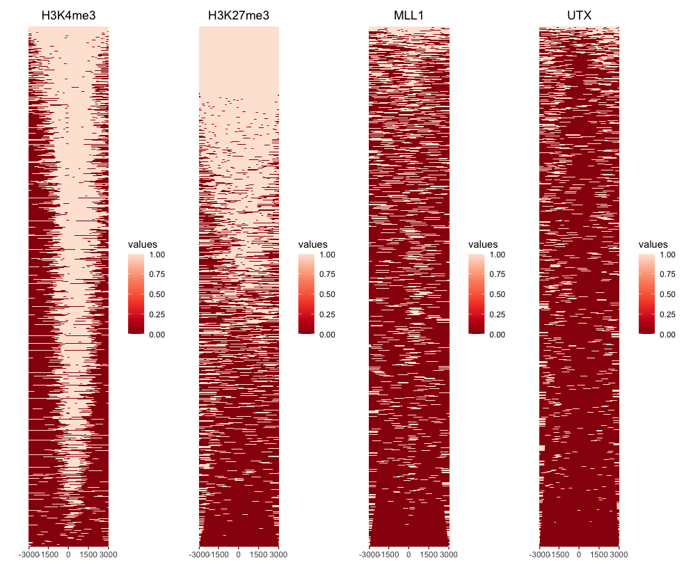
Average Profile of ChIP peaks binding to TSS region
# Multiplot plotAvgProf(tagMatrixList, xlim=c(-3000, 3000), xlab="Genomic Region (5'->3')", ylab = "Read Count Frequency") # Selected plot plotAvgProf(tagMatrixList[c("H3K4me3", "MLL1")], xlim=c(-3000, 3000), xlab="Genomic Region (5'->3')", ylab = "Read Count Frequency") # Selected plot plus confidence interval estimated by bootstrap method plotAvgProf(tagMatrixList[c("H3K4me3", "MLL1")], xlim=c(-3000, 3000), xlab="Genomic Region (5'->3')", ylab = "Read Count Frequency", conf = 0.95, resample = 1000) # facet plotAvgProf(tagMatrixList, xlim=c(-3000, 3000), xlab="Genomic Region (5'->3')", ylab = "Read Count Frequency", conf = 0.95, resample = 500, facet = "row")- Output:
  > plotAvgProf(tagMatrixList[c("H3K4me3", "MLL1")], xlim=c(-3000, 3000), xlab="Genomic Region (5'->3')", ylab = "Read Count Frequency",conf = 0.95, resample = 1000)
  >> plotting figure...			 2024-05-21 16:15:42
  >> Running bootstrapping for tag matrix...		 2024-05-21 16:17:15
  >> Running bootstrapping for tag matrix...		 2024-05-21 16:17:34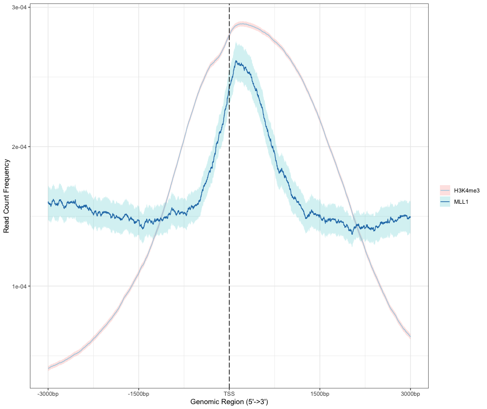
Adding your own Transcript Database(Txdb)
Species that are less commonly studied often do not have associated database packages in R. In such cases, it is possible to extract the Txdb simply using
makeTxDbFromGFFfunction from the GTF file. In this context, I will use the rice genome as an example to demonstrate the extraction method.gtf_file <- "/Users/jchoi/Desktop/IRGSP.gtf" txdb <- makeTxDbFromGFF(gtf_file)
5. Peak Annotation
- The
annotatePeakfunction in the ChIPseeker package is used to annotate peaks in ChIP-seq data analysis. The function identifies and annotates where peaks map to functional elements of the genome, such as promoters, UTRs (5 and 3), exons, introns, intergenic, and downstream regions.peakAnnoList <- lapply(peaks, annotatePeak, TxDb=txdb, tssRegion=c(-3000, 3000), addFlankGeneInfo=TRUE, flankDistance=5000, annoDb="org.Hs.eg.db") peakAnnoList # Check resultsIn these arguments,
Parameter Description peaksThe list of peak files provided as the first argument to the lapplyfunction.TxDbTranscript Database (TxDb) object. tssRegionThe distance range from the TSS. The default is c(-3000, 3000), which means peaks will be annotated within 3000 base pairs upstream and downstream of the TSS.addFlankGeneInfoSpecifies whether to add information about genes flanking the peaks. Setting this to TRUEwill include information about genes located upstream and downstream of the peaks.flankDistanceSpecifies the distance upstream and downstream to include when adding flanking gene information. The default is 5000 base pairs. annoDbSpecifies annotation database. paletteColor palette for the heatmap.
Output:
  > peakAnnoList <- lapply(peaks, annotatePeak, TxDb=txdb, tssRegion=c(-3000, 3000),
  +                        addFlankGeneInfo=TRUE, flankDistance=5000, annoDb="org.Hs.eg.db")
      >> preparing features information...		 2024-05-21 16:51:05
      >> identifying nearest features...		 2024-05-21 16:51:06
      >> calculating distance from peak to TSS...	 2024-05-21 16:51:06
      >> assigning genomic annotation...		 2024-05-21 16:51:06
      >> adding gene annotation...			 2024-05-21 16:51:17
      'select()' returned 1:many mapping between keys and columns
      >> adding flank feature information from peaks...	 2024-05-21 16:51:18
      >> assigning chromosome lengths			 2024-05-21 16:51:26
      >> done...					 2024-05-21 16:51:26

  > peakAnnoList
  $H3K4me3
  Annotated peaks generated by ChIPseeker
  59582/59583  peaks were annotated
  Genomic Annotation Summary:
              Feature   Frequency
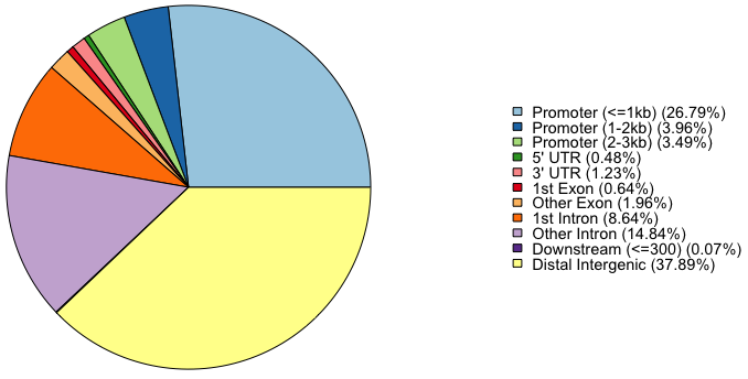
  9    Promoter (<=1kb) 26.79332684
  10   Promoter (1-2kb)  3.96092780
  11   Promoter (2-3kb)  3.49434393
  4              5' UTR  0.47665402
  3              3' UTR  1.22855896
  1            1st Exon  0.64113323
  7          Other Exon  1.96032359
  2          1st Intron  8.64355007
  8        Other Intron 14.83501729
  6  Downstream (<=300)  0.07384781
  5   Distal Intergenic 37.89231647

  ====================(skip)========================

  $UTX
  Annotated peaks generated by ChIPseeker
  44844/44845  peaks were annotated
  Genomic Annotation Summary:
              Feature  Frequency
  9    Promoter (<=1kb)  3.1375435
  10   Promoter (1-2kb)  3.3850682
  11   Promoter (2-3kb)  3.1643029
  4              5' UTR  0.4147712
  3              3' UTR  1.2576933
  1            1st Exon  0.3255731
  7          Other Exon  3.0171260
  2          1st Intron 10.2600125
  8        Other Intron 27.2277228
  6  Downstream (<=300)  0.1204174
  5   Distal Intergenic 47.6897690
Save annotated peaks as the csv format as follow:
  write.csv(peakAnnoList[["H3K4me3"]], "Peaked_H3K4me3.csv")
  write.csv(peakAnnoList[["H3K27me3"]], "Peaked_H3K27me3.csv")
  write.csv(peakAnnoList[["MLL1"]], "Peaked_MLL1.csv")
  write.csv(peakAnnoList[["UTX"]], "Peaked_UTX.csv")
6. Visulize genomic annotation
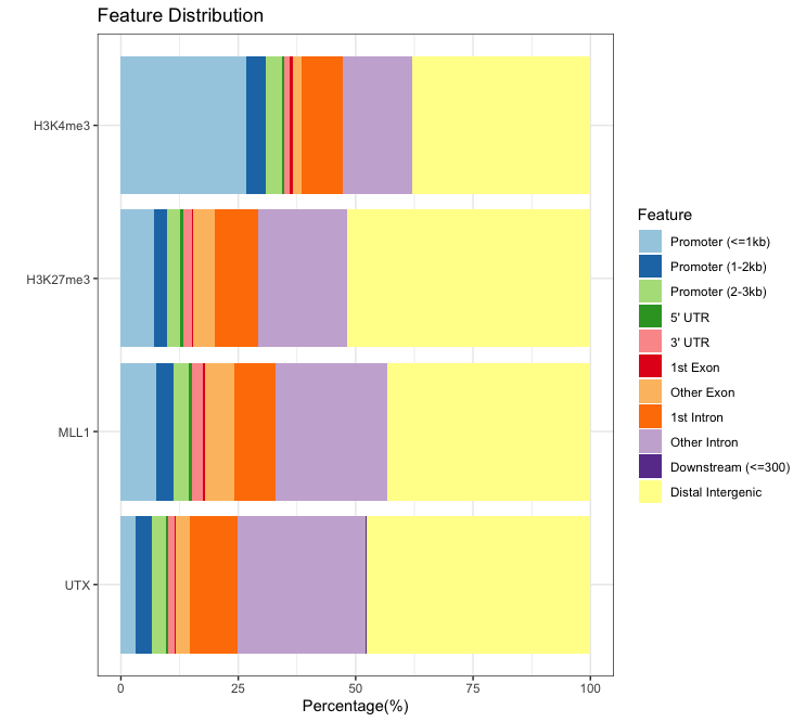
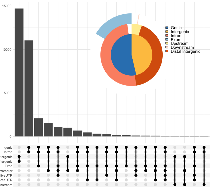
- Finally, I will discuss and visualize where the annotated peaks are located in the genomic regions, including promoters, UTRs (5 and 3), exons, introns, intergenic, and downstream regions.
- Pie plot: This funtion does not provide drawing multiplot.
  plotAnnoPie(peakAnnoList[["PeakName"]]) # PeakName is an assigned peak name using the list function

  # For example
  plotAnnoPie(peakAnnoList[["H3K4me3"]]) # Ouput
Output:
- Bar plot
  plotAnnoBar(peakAnnoList) # Multiplot, output
  plotAnnoBar(peakAnnoList[["PeakName"]]) # Indivisual plot
Output:
- Vennpie plot: This funtion does not provide drawing multiplot.
vennpie(peakAnnoList[["PeakName"]]) - UpSet plot: This funtion does not provide drawing multiplot.
upsetplot(peakAnnoList[["PeakName"]], vennpie = TRUE) # TRUE/FALSE: with/without vennpie, outputOutput:
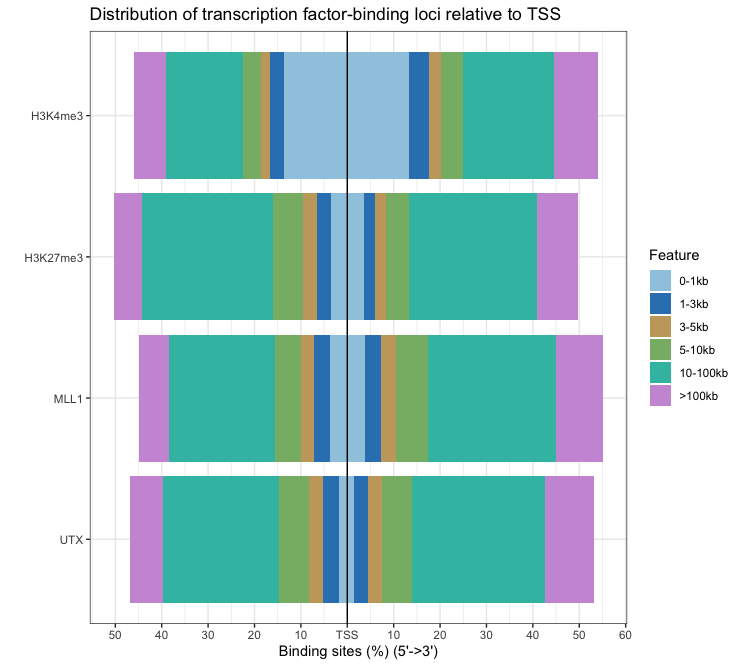
- Distribution of TF-binding loci relative to TSS: The distance from the peak (binding site) to the TSS of the nearest gene is calculated by annotatePeak and reported in the output.
  plotDistToTSS(peakAnnoList) # output
  plotDistToTSS(peakAnnoList[["PeakName"]])
Output:
- The functions
bdgdiffin MACS3 andsicer-dfin SICER2 produce results using the same annotation method (annotatePeak). - Although HOMER's
annotatePeaks.plcan be used for annotation, it is rarely employed currently. - Peak distribution analysis, including heatmaps and average plots, can be effectively performed with both
deeptoolsandngsplot. I recommendngsplotfor optimal results. - Peak feature analysis (Section 6, visualization) is seldom used unless investigating a novel transcription factor via ChIP-seq.
- Despite detailed peak analysis, the current trend focuses on identifying meaningful genes from the detected peaks.
Citation
- Yu, G., Wang, L. G., & He, Q. Y. (2015). ChIPseeker: an R/Bioconductor package for ChIP peak annotation, comparison and visualization. Bioinformatics, 31(14), 2382-2383. DOI


